這是給自己的一份學習紀錄,以免日子久了忘記這是甚麼理論XD
這篇文章利用 Chat Gpt 翻譯成英文,邊唸邊打(純手打,無複製貼上),順便練英文 XD
We can assume that the data comes from a sample with a normal distribution, in this context, the eigenvalues asyptotically follow a normal distribution. Therefore, we can estimate the 95% confidence interval for each eigenvalue using the following formula: $$ \left[ \lambda_\alpha \left( 1 - 1.96 \sqrt{\frac{2}{n-1}} \right); \lambda_\alpha \left(1 + 1.96 \sqrt{\frac{2}{n-1}} \right) \right] $$ where:
- $\lambda_\alpha$ represents the $\alpha$-th eigenvalue
- $n$ denotes the sample size.
By caculating the 95% confidence intervals of the eigenvalue, we can assess their stability and determine the appropriate number of pricipal component axes to retain. This approach aids in deciding how many principal components to keep in PCA to reduce data dimensionality while preserving as much of the original information as possible.
In PCA, it’s typically assumed that variables are continuous and follow a normal distribution. However, the presence of outliers or extreme values can violate these assumptions, potentially affecting the analysis results. To moderate these effects, data trasformation can be considered to make the results independent of measurement scales and monotonic transformations. A commone method is to replace each observation with its rank within the variable. In rank transformation, Spearman’s rank corrlelation coefficient is often used to measure the monotonic relationship between two variables. The calculation formula is: $$ r_s\left(j, j'\right) = 1 - \frac{6\sum_{i=1}^n \left(x_{ij} - x_{ij'}\right)^2}{n(n^2-1)} $$ where:
- $r_s\left(j, j^’\right)$ denotes the Spearman correlation coefficient between variables $j$ and $j'$
- $x_{ij}$ and $x_{ij^’}$ represent the ranks of the $i$-th observation in variables $j$ and $j'$
- $n$ is the total number of observations
Spearman rank transformation offers several keys advantages:
- Reducing the impact of outliers
- Preserving the ‘relative relationships’ between variables while ignoring data units
- Capturing non-linear relationships
Relationship between PCA and clustering ayalysis
PCA for dimensionality reduction enhances clustering effectiveness
Challenge in high-dimensional data & Solution Through PCA
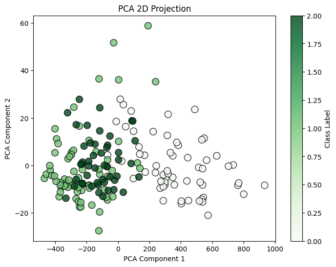
Clustering algorithms can be adversely affected by the ‘Curse of Dimensionality’ when dealing with high-dimensional datasets, by applying PCA for dimensionality reduction, we can project data into a lower-dimentional space(e.g. 2D), facilitating more stable and interpretable clustering results.
To discover clusters of data points that share similar characteristics, common clustering techniques include:
- Hierachical clustering: Generates a dendrogram to represent nested groupings of data points.
- K-means clustering: Partitions data points into k clusters based on proximity to cluster centroids.
Applications of PCA and Clustering:
- Market Segmentation: Classifying consumers based on purchasing behavior to tailor marketing strategies.
- Medical Data Analysis: Identifying patient subgroups to enhance personalized treatment plans.
- Socioeconomic Studies: Analyzing patterns of economic development across different urban areas.
- Gene Expression Analysis: Detecting groups of genes with similar expression profiles to understand biological processes.
In PCA, the inclusion of weights can influence the calculation of means, covariances, and correlations. Unweighted analyses focus on describing the sample, whereas weighted analyses aim to infer characteristics of the overall population. Therefore, when assigning weights, it’s crucial to avoid excessive variability and consider them carefully to encure the stability and reliability of the estimates.
We need to express the response variable in terms of the original variables. Each principal component is written as a linear combination of the explanatory variables: $$y = b_o + b_1\Psi_1 + \cdots + b_p\Psi_p = \hat{\beta}_0 + \hat{\beta}_1x_1 + \cdots $$ Selecting prinicpal components with eigenvalues significantly greater than 0 as new explanatory variables can enhance the model’s stability and interpretability. This approach ensures that each retained component accounts for a substantial protion of the data’s variance, leading to more reliable and meaningful results.
When we lack a variable matrix X and only have an inter-individual distance matrix D, we can still perform PCA using inner product matrix transformation, similar to the concept of Multidimensional Scaling(MDS).
In what situations do we only have distance between individuals?
In many real-world scenarious, data is not presented as a clear variable matrix X but exits in the form of a distance matrix. Here are some examples:
1. Similarity/Dissimilarity Matrices
- Genetic Research: The similarity between DNA sequences can be converted into Euclidean or Jaccard distances.
- Text Mining: The similarity between documents can be calculated using Cosine Similarity or Edit Distance.
2. Social Network Analysis
- The number of mutual friends can define a similarity matrix, which can then be converted into distances.
- Message transmission time can represent the ‘distance’ between individuals.
3. Geospatial & Transportation Data
- Urban Planning: Distances between cities can be used in PCA to help identify regional clusters.
- Applications like Google Maps: Analyzes similarities between cities using actual route distances.
4. Recommendation Systems
- In e-commerce or music recommendation systems, user behavior can be measured by ‘distance’.
- The more similar the products purchased by two users, the shorted the ‘distance’ between them.
When we have only the inter-individual matrix D, we can transform it into an inner product matrix W using the following formula: $$w_{il} = \frac{1}{2} \left( d^2_{i\cdot} + d^2_{l\cdot} - d^2_{\cdot\cdot} - d^2{(i, l)} \right)$$ where:
- $d^2{(i, l)}$ represents the squared distance between individuals $i$ and $l$
- $d^2_{i\cdot}$ and $d^2_{l\cdot}$ are the average squared distances of individuals $i$ and $l$ to all other individuals
- $d^2_{\cdot\cdot}$ is the overall average of these squared distances
After obtaining the inner product matrix W, we can perform PCA by applying eigenvalue decomposition or SVD to W for dimensionality reduction.
And here is the different between eigenvalue decomposition and SVD
| Condition | Eigen Decomposition | SVD |
|---|---|---|
| Matrix Type | Only for square matrices | Can be applied to any matrix shape |
| Applicable To | Inner product matrix $W$, covariance matrix $C$ | Original data matrix $X$ |
| Data Size | Best for $p \ll n$ | Best for $p \gg n$ |
| Results | Obtains principal component directions( variable correlations ) | Obtains both individual projections and principal components |
| Computational Efficiency | More computationally expensive( requires computing $C$ ) | More efficient, suitable for high-dimensional data |
In practical applications, libraries like scikit-learn implement PCA using SVD, as it is more numerically stable and computaionally efficient.
Conditional PCA
By incorporating matrix $Z$ to control for certain variables, we can analyze the variability in the data using the residual matrix $E$. The matrix $Z$ represents grouping information, such as: controlling for time effects, eliminating the influence of income, analyzing results based on PCA, or grouping based on categories. The residual matrix $E$ allows us to assess the variability of variables after accounting for specific influencing factors( represented by matrix $Z$ ). The formula for the residual matrix $E$ is:
$$
\frac{1}{n} E^T E = \frac{1}{n} \left( X^TX - X^TZ(X^TX)^{-1}Z^TX \right) = V(X|Z)
$$
This method calculates the after removing the effects of conditional variables. The goal is to eliminate the influence of certain known factors and focus on unexplained variability. This approach is widely applied in fields such as finance, social sciences, bioinformatics, and time series analysis.
Regardless of the utilized medthod for modeling the variables $X$, we always decompose the covariance matrix into two terms: one term explains the variables $Z$, whose effect we want to elimate; the other term expresses the remaining or residual variability. The conditional analysis involves analyzing this latter term $$ V = V_{explained} + V_{residual} $$