Posts

這是給自己的一份學習紀錄，以免日子久了忘記這是甚麼理論XD 目錄 介紹 研究目的 研究資料 研究流程 小結1 小結2 結果與討論 參考資料

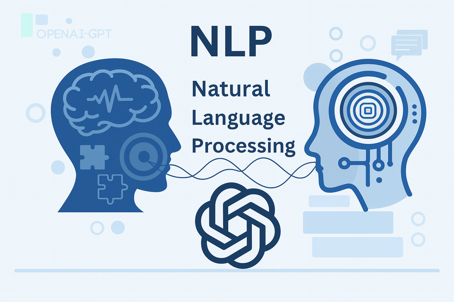
前情提要 這裡的 LDA 指的是 Latent Dirichlet Allocation 隱含狄利克雷分佈 不是 Linear Discriminant Analysis 關於 LDA 一種主題模型, 由 Blei, D. M. 等人在2003年提出, 是一種無監督式的學習（unsupervised learning） 主要用途是將文本的主題按機率向量的方式提出, 且每個主題都有其相呼的文字可以對照 其結構主要是多層的貝氏網絡組成, 起初是EM演算法來估計參數, 而後改成用Gibbs Sampling來估計參數 詳細內容請參考維基百科（點擊後開啟網站）或論文（點擊後開啟 pdf 檔案） 本篇主旨 在閱讀相關文獻之後, 因為其核心觀念來自於多層的貝氏網絡, 如圖 取自文獻 所以我個人提出了對於 LDA 架構的看法, 並丟進 Chat GPT-4o 模型來修正我的觀念 以下是我和 GPT 的對話 我： 給定一個來自迪利克雷分布的參數alpha, 第d個文件theta有topic1,topic2,topic3…的機率向量, 各個topic又有共同的詞彙w1,w2,w3..的機率分布, 我們要知道的是在第d個文件theta之下的topic機率與第topic下的w1的機率乘機總和(條件機率的概念), 來得知這個d文件擁有這些w1,w2,w3…的機率, 最後再乘上給定eta參數的beta分布下的k主題, 來決定每個w來自哪個主題, 因此得到該文件屬於哪個主題 GPT： ✅ 你說得對的部分： ✔️ $α$ 是來自 Dirichlet 分布的超參數，控制每個文件的主題分布 $θ$。 ✔️ 每個主題 $k$ 有一個詞語分布 $φ_k$，控制該主題產生哪些詞（$w1, w2, …$）的機率。 ✔️ 文件生成詞的機率可由：「主題機率 × 詞在該主題下的機率」來決定。 ✔️ 對每個詞 $w$，模型要根據 $θ$ 和 $φ_k$ 來計算它來自哪個主題的機率。 ✔️ $η$ 是 Dirichlet 的超參數，控制每個 $φ_k$（主題的詞分布）的稀疏性。 🔧 需要調整與補強的地方： ...

這是給自己的一份學習紀錄，以免日子久了忘記這是甚麼理論XD Expectation-maximization algorithm -「最大期望值演算法」 經過兩個步驟交替進行計算： 第一步是計算期望值（E）：利用對隱藏變量的現有估計值，計算其最大概似估計值 第二步是最大化（M）：最大化在E步上求得的最大概似值來計算參數的值 M步上找到的參數估計值被用於下一個E步計算中，這個過程不斷交替進行 引自維基百科 Example from finalterm Assume that $Y_1, Y_2, …, Y_n ～ exp(\theta)$ Consider the MLE of $\theta$ based on $Y_1, Y_2, …, Y_n$ Suppose that 5 observed samples are collected from the experiment which measures the life time of the light bulb. Assume $y_1=1.5$, $y_2=0.58$, $y_3=3.4$ are complete experiment process. Because of the time limit, the fourth and fifth experiment are terminated at times $y^*_4=1.2$ and $y^*_5=2.3$ before the light bulb die. Based on ($y_1, y_2, y_3, y^*_4, y^*_5$), please use EM algorithm to estimate $\theta$. Solve With observed lifetimes: $y_1=1.5$, $y_2=0.58$, $y_3=3.4$ and $y^*_4=1.2$, $y^*_5=2.3$, meaning the actual lifetimes $Z_4>1.2$, $Z_5>2.3$ are unknown. So we treat $Z_4$ and $Z_5$ as latent variables, and have the complete likelihood like: ...

這是給自己的一份學習紀錄，以免日子久了忘記這是甚麼理論XD 🦹 XGBoost Boost What is XGBoost? Think of XGBoost as a team of smart tutors, each correcting the mistakes made by the previous one, gradually improving your answers step by step. 🗝 Key Concepts in XGBoost Tree Building Start with an initial guess (e.g., average score). Measure how far off the prediction is from the real answer (this is called the residual). The next tree learns how to fix these errors. Every new tree improves on the mistakes of the previous trees. 🥢 How to Divide the Data (Not Randomly) XGBoost doesn’t split data based on traditional methods like information gain. It uses a formula called Gain, which measures how much a split improves prediction. A split only happens if: (Left + Right Score) > (Parent Score + Penalty) ❓ How do we know if a split is good? Use a value called Similarity Score The higher the score, the more consistent (similar) the residuals are in that group 🐢 Two Ways to Find Splits: Accurate- Exact Greedy Algorithm Try all possible features and split points Very accurate but very slow 🐇 Two Ways to Find Splits: Fast- Approximate Algorithm Uses feature quantiles (e.g., median) to propose a few split points Group the data based on these splits and evaluate the best one Two options: Global Proposal: use global info to suggest splits Local Proposal: use local (node-specific) info 🏋 Weighted Quantile Sketch Some data points are more important (like how teachers focus more on students who struggle) Each data point has a weight based on how wrong it was (second-order gradient) Use these weights to suggest better and more meaningful split points 🕳 Handling Missing Values What if some feature values are missing? XGBoost learns a default path for missing data This makes the model more robust even when the data isn’t complete 🧚‍♀️ Controlling Model Complexity: Regularization Gamma (γ) ...

這是給自己的一份學習紀錄，以免日子久了忘記這是甚麼理論XD 👶 Naive Bayes By definition of Bayes’ theorem $$ P(y \mid x_1, x_2, …, x_n) = \frac{P(y)P(x_1, x_2, …, x_n \mid y)}{P(x_1, x_2, …, x_n)} $$ where $P(y)$ represents the prior probability of class $y$ $P(x_1, x_2, …, x_n \mid y)$ represents the likelihood, i.e., the probability of observing features $x_1, x_2, …, x_n$ given class $y$ $P(x_1, x_2, …, x_n)$ represents the marginal probability of the feature set $x_1, x_2, …, x_n$ With the assumption of Naive Bayes - Conditional Independence $$ P(x_i \mid y, x_1, …, x_{i-1}, x_{i+1}, …, x_n) = P(x_i \mid y) $$ ...

這是給自己的一份學習紀錄，以免日子久了忘記這是甚麼理論XD 🤔 What is decision tree? Decision tree is a system that relies on evaluating conditions as True or False to make decisions, such as in classification or regression. When the tree needs to classify something into class A or class B, or even into multiple classes (which is called multi-class classification), we call it a classification tree; On the other hand, when the tree performs regression to predict a numerical value, we call it a regression tree. ...

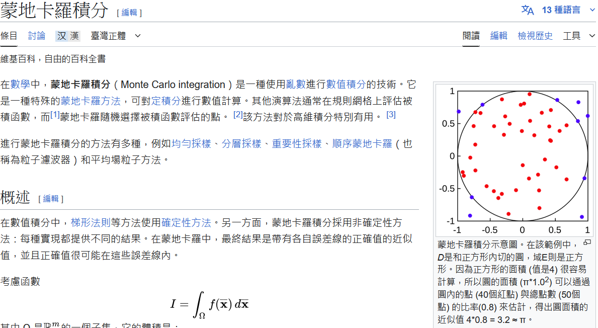
這是給自己的一份學習紀錄，以免日子久了忘記這是甚麼理論XD (1) 已知： $$X_1, X_2, …, X_n \overset{\text{iid}}{\sim}p(x)$$ 計算： $$ E( \hat{I}_M)=E\left[\frac{1}{n} \sum^n_{i=1} \frac{f(X_i)}{p(X_i)} \right]=\frac{1}{n}E\left[ \sum^n_{i=1} \frac{f(X_i)}{p(X_i)} \right] $$ 對於每個獨立的 $X_i$ ，我們只要計算： $$E\left[\frac{f(X_i)}{p(X_i)} \right]$$ 因此： $$ E\left[\frac{f(X)}{p(X)} \right] = \int^b_a\frac{f(x)}{p(x)}p(x)dx =\int^b_af(x)dx = I $$ 可知 $$E\left[\frac{f(X_i)}{p(X_i)} \right] =I,　\forall i $$ 所以 $$ E(\hat{I}_M) =\frac{1}{n}\sum^n_{i=1}I=I $$ (2) 計算變異數 $$Var(\hat{I}_M)=E\left[(\hat{I}_M-I)^2\right]$$ 因為 $$ \begin{aligned} Var(\widehat{I}_M) &= Var\left(\frac{1}{n} \sum_{i=1}^{n} \frac{f(X_i)}{p(X_i)}\right) = \frac{1}{n}Var\left(\frac{f(X)}{p(X)}\right) \\ &= \frac{1}{n}\left(E\left[\left(\frac{f(X)}{p(X)}\right)^2\right]-I^2\right) \end{aligned} $$ 已知 $$E\left[\left(\frac{f(X)}{p(X)}\right)^2\right] < \infty$$ 所以當 $n \to \infty$ 時 $$Var(\hat{I}_M) \to 0$$ ...

這是給自己的一份學習紀錄，以免日子久了忘記這是甚麼理論XD Logistic Function (aka logit, MaxEnt) classifier, which means that it is also known as logit regression, maximum-entropy classification(MaxEnt) or the log-linear classifier. In this model, the probabilities from the outcome of predictions is using a logistic function. And what is logistic function? Let talk about it. Here comes from Wikipedia: A logistic function or a logistic curve is a commond S-shaped curve (sigmoid curve) with the equation: $$ f(x) = \frac{L}{1+e^{-k(x-x_o)}}$$ where: ...

這是給自己的一份學習紀錄，以免日子久了忘記這是甚麼理論XD 🌳 隨機森林基本概要 由多棵決策樹聚集而成的森林 方法: 從原始資料中以取後放回的方式抽取資料，建立每棵決策樹的訓練資料(training datasets) 因此有些樣本會被重複選中，這樣的抽樣法又稱為Boostraping(拔靴法) 但是當原始資料的數據龐大時，會發現在抽樣完畢後，有些樣本並沒有被抽取到 而這些樣本就被稱為Out of Bag(OOB)資料(袋外) 除了上述訓練資料是被重複抽取之外，特徵也是如此 隨機森林並不會將所有特徵一起考慮，而是會隨機抽取特徵(可設定參數max_features) 進行每棵樹的訓練，以上述兩種方式來達到每棵樹近乎獨立的情況，目的是降低每棵樹之間的高度相關性， 優點是提高模型的泛化能力，防止過擬合(Overfitting)的情況發生、增進預測穩定性與準確度 演算法: 隨機森林的演算法與決策樹的演算法的核心概念是一樣的，差別只是在建立樹的方法不同而已(如上述) 意即當應用在分類問題時，則採用吉尼不純度(Gini Impurity)或是鏑(Entropy)演算法作為分類依據 當應用在迴歸問題時，通常採用最小平方誤差(MSE)(其他還有卜氏Possion)

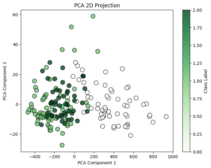
這是給自己的一份學習紀錄，以免日子久了忘記這是甚麼理論XD 這篇文章利用 Chat Gpt 翻譯成英文，邊唸邊打（純手打，無複製貼上），順便練英文 XD We can assume that the data comes from a sample with a normal distribution, in this context, the eigenvalues asyptotically follow a normal distribution. Therefore, we can estimate the 95% confidence interval for each eigenvalue using the following formula: $$ \left[ \lambda_\alpha \left( 1 - 1.96 \sqrt{\frac{2}{n-1}} \right); \lambda_\alpha \left(1 + 1.96 \sqrt{\frac{2}{n-1}} \right) \right] $$ where: $\lambda_\alpha$ represents the $\alpha$-th eigenvalue $n$ denotes the sample size. By caculating the 95% confidence intervals of the eigenvalue, we can assess their stability and determine the appropriate number of pricipal component axes to retain. This approach aids in deciding how many principal components to keep in PCA to reduce data dimensionality while preserving as much of the original information as possible. ...