這是給自己的一份學習紀錄,以免日子久了忘記這是甚麼理論XD
Logistic Function (aka logit, MaxEnt) classifier, which means that it is also known as logit regression,
maximum-entropy classification(MaxEnt) or the log-linear classifier.
In this model, the probabilities from the outcome of predictions is using a logistic function.
And what is logistic function?
Let talk about it.
Here comes from Wikipedia:
A logistic function or a logistic curve is a commond S-shaped curve (sigmoid curve) with the equation: $$ f(x) = \frac{L}{1+e^{-k(x-x_o)}}$$ where:
- $L$ is the supremum of the values of the function
- $k$ is the logistic growth rate, the steepness of the curve
- $x_0$ is the $x$ value of the function’s midpoint
中譯:
- $L$ 是該函數(系統)一個最大上限,當 $x \to 0$ 時,則 $ f(x) \to L$
- $k$ 該曲線的陡峭程度,$k$ 愈小則分母愈大,整個 $f(x)$愈小,表示中間變化速度緩慢;反之則中間變化速度快
- $x_0$ 曲線當中變化速度最快的一點
我們可以簡化該方程式:
The standard logistic function, where $L=1, k=1, x_0=0$, has the euqation: $$ f(x) = \frac{1}{1+e^{-x}}$$
and is also called sigmoid function, and it looks like:
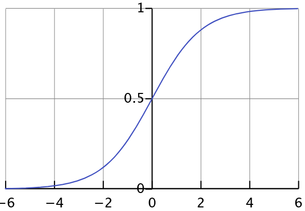 We can know that:
- When $x=0, f(0)= \frac{1}{2}$
- When $x=\infty, f(\infty)= 1$
- When $x=-\infty, f(-\infty)=0$
Therefore, we use this function because the logistic function ranges between 0 and 1 and is relatively simple among smooth functions
But how does logistic regression find the best estimators for making predictions?
Here is the process
1. Target
We suppose that: $$ f(X) = P(Y=1 \mid X) = \frac{1}{1+e^{-(W^TX)}} $$ and we should know that:
$$ P(Y\mid X) = f(X) \text{if } Y=1 $$
$$ P(Y\mid X) = 1 - f(X) \text{if } Y=0 $$
2. How to
Logistic regression uses the likelihood function to estimate parameters, allowing the model to make more precise predictions. So we define likelihood function: $$ L(W, b) = \Pi^n_{i=1}P\left(y_i \mid x_i \right) $$
3. Mathematical
Then we plug $P(Y\mid X)$ into the formula, so we have: $$ L(W, b) = \Pi^n_{i=1}\left(\frac{1}{1+e^{-(W^TX)}}\right)^{y_i}\left(1-\frac{1}{1+e^{-(W^TX)}}\right)^{1- y_i} $$ and we take the log of likelihood function(log-likelihood): $$ lnL(W, b) = \Sigma^n_{i=1}\left[y_iln\left(\frac{1}{1+e^{-(W^TX)}}\right)\right] + (1- y_i)ln\left(1-\frac{1}{1+e^{-(W^TX)}}\right)$$
then we use calculus and gradient descent to find the optimal parameter W. Finally, we ensure that the likelihood function reaches its maximum, which corresponds to the MLE solution.
In my opinion
It is easy to see that using linear regression for predicting or classifying binary classes can be highly influenced by outliers.
A small change in the data can cause a data point to switch from Class 1 to Class 2 unpredictably, which is unreasonable.
To address this issue and improve the regression model for binary classification, we use a logistic function that better fits the binary class data.
🔧 Modeling with sklearn.LogisticRegression
import pandas as pd
import seaborn as sns
import numpy as np
import matplotlib.pyplot as plt
coloumns_name = ['Length', 'Left', 'Right', 'Bottom', 'Top', 'Diagonal']
data = pd.read_csv('bank2.dat', delim_whitespace=True, header=None, names=coloumns_name)
data.head()
--------------------------------------------------
   Length   Left  Right  Bottom   Top  Diagonal    Class
0   214.8  131.0  131.1     9.0   9.7     141.0  Genuine
1   214.6  129.7  129.7     8.1   9.5     141.7  Genuine
2   214.8  129.7  129.7     8.7   9.6     142.2  Genuine
3   214.8  129.7  129.6     7.5  10.4     142.0  Genuine
4   215.0  129.6  129.7    10.4   7.7     141.8  Genuine
data.info()
--------------------------------------------------
<class 'pandas.core.frame.DataFrame'>
RangeIndex: 200 entries, 0 to 199
Data columns (total 7 columns):
 #   Column    Non-Null Count  Dtype
---  ------    --------------  -----
 0   Length    200 non-null    float64
 1   Left      200 non-null    float64
 2   Right     200 non-null    float64
 3   Bottom    200 non-null    float64
 4   Top       200 non-null    float64
 5   Diagonal  200 non-null    float64
 6   Class     200 non-null    object
dtypes: float64(6), object(1)
memory usage: 11.1+ KB
data.isna().sum()
--------------------------------------------------
Length      0
Left        0
Right       0
Bottom      0
Top         0
Diagonal    0
Class       0
dtype: int64
data.describe().T
--------------------------------------------------
          count      mean       std    min    25%     50%      75%    max
Length    200.0  214.8960  0.376554  213.8  214.6  214.90  215.100  216.3
Left      200.0  130.1215  0.361026  129.0  129.9  130.20  130.400  131.0
Right     200.0  129.9565  0.404072  129.0  129.7  130.00  130.225  131.1
Bottom    200.0    9.4175  1.444603    7.2    8.2    9.10   10.600   12.7
Top       200.0   10.6505  0.802947    7.7   10.1   10.60   11.200   12.3
Diagonal  200.0  140.4835  1.152266  137.8  139.5  140.45  141.500  142.4
from sklearn.model_selection import train_test_split
from sklearn.preprocessing import StandardScaler, LabelEncoder
from sklearn.linear_model import LogisticRegression
from sklearn.metrics import confusion_matrix, accuracy_score, classification_report

X = data.drop(columns=['Class'])
y = data['Class']

X_train, X_test, y_train, y_test = train_test_split(X, y, random_state=42, test_size=0.2)

scaler = StandardScaler()
X_train_scaled = scaler.fit_transform(X_train)
X_test_scaled = scaler.transform(X_test)

lr = LogisticRegression(random_state=42, penalty=None)
model = lr.fit(X_train_scaled, y_train)

y_pred = model.predict(X_test_scaled)
y_proba = model.predict_proba(X_test_scaled)
print(confusion_matrix(y_test, y_pred))
print(accuracy_score(y_test, y_pred))
--------------------------------------------------
[[19  0]
 [ 1 20]]
0.975
print("\nModel Accuracy:", model.score(X_test_scaled, y_test))

print(classification_report(y_test, y_pred))

Model Accuracy: 0.975

              precision    recall  f1-score   support

 Counterfeit       0.95      1.00      0.97        19
     Genuine       1.00      0.95      0.98        21

    accuracy                           0.97        40
   macro avg       0.97      0.98      0.97        40
weighted avg       0.98      0.97      0.98        40
🔨 Modleing with statsmodels.Logit
note:
因為使用該模型存在beta不收斂的問題
所以在fit的部分選擇使用fit_regularized
其中method設定加入l1懲罰, alpha(l1的權重)設0.01
summay才會正常跑出數值
constant = sm.add_constant(X)

model = sm.Logit(y, constant)
result = model.fit_regularized(method='l1', alpha=0.01)

print(result.summary())
--------------------------------------------------
Optimization terminated successfully    (Exit mode 0)
            Current function value: 0.002174041962487562
            Iterations: 131
            Function evaluations: 136
            Gradient evaluations: 131
                           Logit Regression Results
==============================================================================
Dep. Variable:                      y   No. Observations:                  200
Model:                          Logit   Df Residuals:                      193
Method:                           MLE   Df Model:                            6
Date:                Thu, 20 Mar 2025   Pseudo R-squ.:                  0.9994
Time:                        16:39:59   Log-Likelihood:              -0.083416
converged:                       True   LL-Null:                       -138.63
Covariance Type:            nonrobust   LLR p-value:                 6.587e-57
==============================================================================
                 coef    std err          z      P>|z|      [0.025      0.975]
------------------------------------------------------------------------------
const       7.851e-18   1.11e+04   7.07e-22      1.000   -2.18e+04    2.18e+04
Length        -4.8724     46.740     -0.104      0.917     -96.481      86.737
Left        6.129e-16     83.355   7.35e-18      1.000    -163.372     163.372
Right        -6.8e-16     80.137  -8.49e-18      1.000    -157.066     157.066
Bottom       -11.9135     14.936     -0.798      0.425     -41.187      17.360
Top           -9.3913     15.731     -0.597      0.551     -40.224      21.441
Diagonal       8.9620     10.880      0.824      0.410     -12.362      30.286
==============================================================================

Possibly complete quasi-separation: A fraction 0.95 of observations can be
perfectly predicted. This might indicate that there is complete
quasi-separation. In this case some parameters will not be identified.
c:\Users\USER\anaconda3\Lib\site-packages\statsmodels\base\l1_solvers_common.py:71: ConvergenceWarning: QC check did not pass for 1 out of 7 parameters
Try increasing solver accuracy or number of iterations, decreasing alpha, or switch solvers
  warnings.warn(message, ConvergenceWarning)
c:\Users\USER\anaconda3\Lib\site-packages\statsmodels\base\l1_solvers_common.py:144: ConvergenceWarning: Could not trim params automatically due to failed QC check. Trimming using trim_mode == 'size' will still work.
  warnings.warn(msg, ConvergenceWarning)