
這是給自己的一份學習紀錄,以免日子久了忘記這是甚麼理論XD
- Expectation-maximization algorithm -「最大期望值演算法」
- 經過兩個步驟交替進行計算:
第一步是計算期望值(E):利用對隱藏變量的現有估計值,計算其最大概似估計值
第二步是最大化(M):最大化在E步上求得的最大概似值來計算參數的值 M步上找到的參數估計值被用於下一個E步計算中,這個過程不斷交替進行
引自維基百科
Example from finalterm
Assume that $Y_1, Y_2, …, Y_n ~ exp(\theta)$
- Consider the MLE of $\theta$ based on $Y_1, Y_2, …, Y_n$
- Suppose that 5 observed samples are collected from the experiment which measures the life time of the light bulb. Assume $y_1=1.5$, $y_2=0.58$, $y_3=3.4$ are complete experiment process. Because of the time limit, the fourth and fifth experiment are terminated at times $y^*_4=1.2$ and $y^*_5=2.3$ before the light bulb die. Based on ($y_1, y_2, y_3, y^*_4, y^*_5$), please use EM algorithm to estimate $\theta$.
Solve
With observed lifetimes: $y_1=1.5$, $y_2=0.58$, $y_3=3.4$ and $y^*_4=1.2$, $y^*_5=2.3$, meaning the actual lifetimes $Z_4>1.2$, $Z_5>2.3$ are unknown. So we treat $Z_4$ and $Z_5$ as latent variables, and have the complete likelihood like:
$$ L_{complete}(\theta)=\prod^3_{i=1}f(y_i|\theta)\cdot f(Z_4;\theta)\cdot f(Z_5;\theta) $$ Then we compute the complete log-likelihood:
$$ lnL_{complete}{\theta}=\sum^3_{i=1}lnf(y_i|\theta)+lnf(Z_4;\theta)+lnf(Z_5;\theta)=5ln\theta-\theta(\sum^3_{i=1}y_i+Z_4+Z_5) $$
E-step
Given current estimate $\theta^{(t)}$, we compute the expected log likelihood:
$$ Q(\theta|\theta^{(t)})=E_{Z_4, Z_5|\theta^{(t)}}[lnL_{complete}(\theta)] $$ Since $Z_4, Z_5~Exp(\lambda)$ the conditional expectation is:
$$ E[Z|Z>c]=c+\frac{1}{\theta} $$
Thus:
$$ E[Z_4|Z_4>1.2;\theta^{(t)}]=1.2+\frac{1}{\theta^{(t)}}, E[Z_5|Z_5>2.3;\theta^{(t)}]=2.3+\frac{1}{\theta^{(t)}} $$
M-step
Then we have total expected sum of lifetimes:
$$ E^{(t)}_S=y_1+y_2+y_3+E[Z_4]+E[Z_5]=(1.5+0.58+3.4)+(1.2+\frac{1}{\theta^{(t)}})+(2.3+\frac{1}{\theta^{(t)}}) $$
Now, let maximize $lnL_{complete}(\theta)$ with respect to $\theta$
$$ lnL_{complete}(\theta)=5ln\theta-\theta E^{(t)}_S\implies \frac{dlnLcomplete(\theta)}{d\theta}=\frac{5}{\theta}-E^{(t)}_S\implies\overset{\text{Let}}{=}0\implies\theta^{(t+1)}=\frac{5}{E^{(t)}_S}=\frac{5}{8.98+2/\theta^{(t)}} $$
Therefore, we have EM update formula:
$$ \theta^{(t+1)}=\frac{5}{8.98+2/\theta^{(t)}} $$
And we run the code on python, here is the code
import numpy as np
y = np.array([1.5, 0.58, 3.4])
y4_ = 1.2; y5_ = 2.3
theta = 1; tol = 1e-6; max_iter = 100
theta_values = [theta]
for i in range(max_iter):
    Ez4 = y4_+1/theta; Ez5 = y5_+1/theta # E-step
    theta_new = 5/(np.sum(y)+Ez4+Ez5) # M-step
    theta_values.append(theta_new)
    # 收斂檢查
    if abs(theta-theta_new)<tol:
        break
    theta = theta_new
print(f"Estimated theta after {i+1} iterations: {theta:.6f}")
plt.plot(theta_values, marker='o')
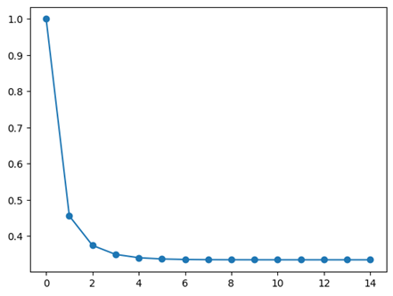
Finally, estimated theta after 14 iterations is 0.334077.
That’s great!!!